Robust control theory was the successor of optimal control theory, and is built around the concept of model uncertainty. Although we have to have some rough idea how the system behaves, we have to accept that our model is imperfect.
Attempting to translate the robust control methodology to economics would be difficult, and I am unsure of its usefulness. I would argue that the main thing to observe is that our analysis of a model should be able to take into account the possibility of other models that can generate similar behaviour, and ask what happens if those models are in fact the correct model. A related secondary issue is the distinction between parameter uncertainty and model uncertainty, which I will discuss here.
(I will note that an attempt to translate robust control to economics was made, but the economists involved decided to stick with a game theoretic version of the theory that has no model uncertainty. The game theoretic version of robust control theory was a novelty that solely existed because of the properties of linear systems, and ignored the concept of model uncertainty.)
Simple Example of Model Uncertainty
The best way to illustrate a concept is with a simple example. However, the need for simplicity means that we need a mathematical example that is divorced from economics (although it does offer insight to the development of robust control theory).
We want to keep a variable x that grows exponentially near zero. The variable grows at a rate of 10% per unit of time (for example, seconds, or months). To make it easy for the reader to re-do the calculations, we will use a discrete time approximation of the continuous time system, with a sample period of .01 time units (seconds).
The equation of motion is:
x[k+1] = x[k] + T(a x[k] + u[k]).
where a is the growth rate (0.1), T is the sample period (.01), and u[k] is the control input. (I am ignoring external disturbances for simplicity). I use square brackets ("[]") to indicate that this is a discrete time system, following electrical engineering convention.
(It will become clear later why I specified the system with a sampling time later.)
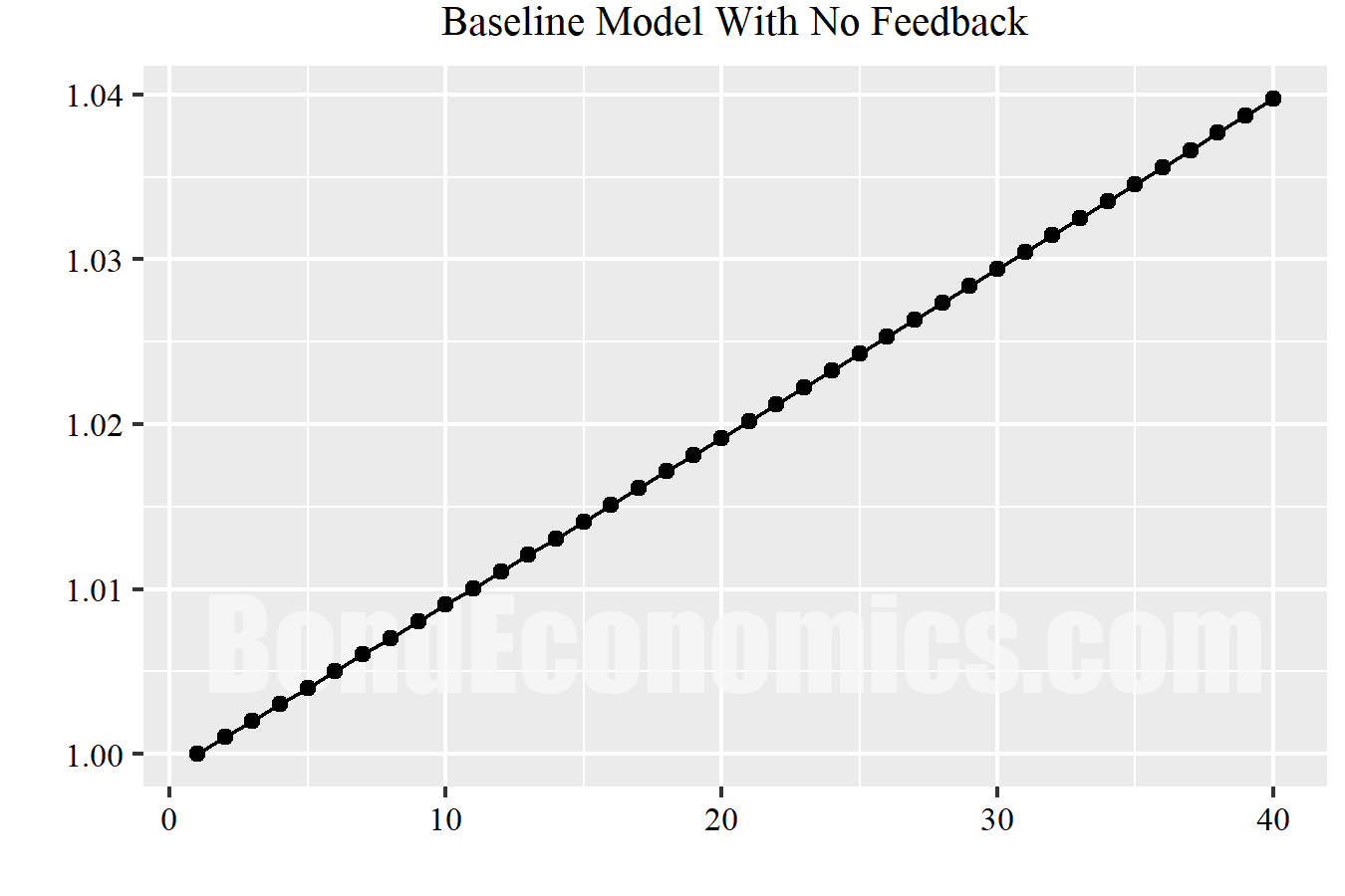
If we set the control input to zero, the system state x follows a steady growth path, as shown above. Note that the time axis is the discrete time period, and not the original time scale.
Let's assume that we use a control law where u is proportional to the variable x (proportional is the P in PID control, a standard form of controller), with a gain of -70 (u[k] = -70 x[k]).
The closed loop has the equation:
x[k+1] = (1 + 0.001 - 0.7)x[k].

The figure above shows what happens when the control law is applied -- the state variable rapidly converges to zero. The second plot shows what happens if we modify the parameter a from 0.1 to 20.1 -- the feedback still drives the state to zero, just slightly slower.
Model Uncertainty Blows Up the Control Law

However, we might be hit by something other than parameter uncertainty. What happens if there is a time delay of 0.02 seconds in reading the output (which is 2 periods). Such a small delay would not be noticeable if one is applying low frequency inputs to the system.
We need to augment our state space model to include two extra variables. The first is the 1-period lag of the state x, and the second is the 1-period lag of the previous variable. The control law is now applied based on the second variable. The figure above shows what happens: the system keeps overshooting zero, and oscillating in an expanding fashion.
This behaviour shows up in a shower with a very sensitive mixing control (or hot water at an unusually high temperature): you need to wait for water to flow through the pipe before adjusting the temperature again, as otherwise you can overshoot. (One standard control laboratory experiment is automatic shower temperature control).
The dangers posed by time delays were one of the key points of failure of optimal control, which is easily illustrated with an example like this. More generally, optimal control was aggressive, and effectively inverted the mathematical of the system to be controlled in order to force the state to follow an optimal trajectory. Inversions are notoriously ill-posed mathematical operations, and this led to dangerous mismatches when applied against real world systems that are not perfectly modelled. (Using the jargon of the field, you could end up with an imperfect pole-zero cancellation, which generates quite unstable dynamics.)
Economics?
The example used is not directly applicable to economics for two reasons.
- Economists are well aware of the concept of policy being subject to uncertain lags.
- Mainstream economists currently focus on monetary policy, where they are largely pushing on a string. Even if one aggressively pushes on a string, it does not matter.
Instead, the issues revolve around analysis. There is a bias for the use of optimisations within modelling, including how to estimate parameters and the state of the economy. This may make techniques vulnerable to outliers (as seen in the effect of 2020 on r* estimates).
More generally, the possibility of models being incorrect are effectively underweighted. The assumption is that prediction errors are the result of external shocks hitting a known model (albeit one with parameter variability), and not the effect of missing dynamics. More specifically, the possibility of the interaction of the preferred methodology with models that do not conform to assumptions is not taken seriously enough.
Really like this post thanks. I used to make similar arguments when discussing option pricing models -- not only about parameter errors but the fact that the entire model is flawed. Btw, do you really believe there is something like r*, or a Wicksellian neutral rate? I think I have given up on this concept.
ReplyDeleteI don’t think it exists. The premise behind r* is that there is a single neutral rate, that is somewhat stable over time. At best, interest rates have different effects on different sectors, and so the effect of rate changes will depend upon the state of each sector.
DeleteEconomists over-complicate things, and refer to this as “multiple equilibria,” which is terrible, given the pseudo-science around the notion of equilibrium.